
In this section, we will be discussing the implementation of some common audio effects, including equalizer, distortion, compressor, limiter, delay and reverb.
Equalizer (EQ)
In the previous section, we implemented a simple low-pass filter. The EQ effector used in the actual mix is much more complicated. It does not simply keep some frequencies and eliminate others. Usually, it requires adjusting the relative strengths and ratios of different frequency bands. Here’s a example:
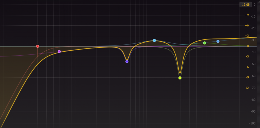
Equalizer, or EQ, adjusts the intensity of different frequency bands by connecting several basic filters in series and parallel.
Common filter types for EQ are low-pass filters (allowing low frequencies to pass), high-pass filters (allowing high frequencies), band-pass filters (allowing a specific frequency range), band-stop filters (preventing a specific frequency from passing), bell filters (enhancing or attenuating a specific frequency range), etc.
For example, when using an equalizer to create a telephone effect, you need to turn on both high cut (low pass) and low cut (high pass) in the equalizer. This essentially means that the signal passes through both filters in series. The process to derive the formula for the high-pass filter is similar. Just write out the circuit, derive the tranfer function, discretize it. Here is the diagram for high-pass RC filter circuit:

This is the frequency response for high-pass RC filter:

The frequency response of the bell filter is as follows, with the amplitude response in blue and the phase response in magenta.

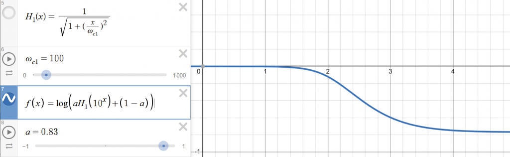
The parallel connection of the filters is also easy to understand. Part of the signal is passed through a low-pass filter, and the other part is left unprocessed. Then we mix both parts. In theory, we should get a response that the high frequency band are partially reduced:
However, there’s a serious problem that we should not ignore: the phase difference. Let’s review the network function of the RC low-pass filter circuit.
$H(jw)=\frac{1}{1+\frac{\omega}{\omega_{c}}}$
In the previous section, we only discussed the change in amplitude. But there’s also a change in phase:
$\theta(\omega)=-arctan(\frac{\omega}{\omega_{c}})$
It is clear that there is a phase shift in the signal after passing through the filter. This shift is nonlinear and varies for different frequencies. If we directly mix the phase-shifted signal with the original signal, the two will interfere and cause a reduction in amplitude.
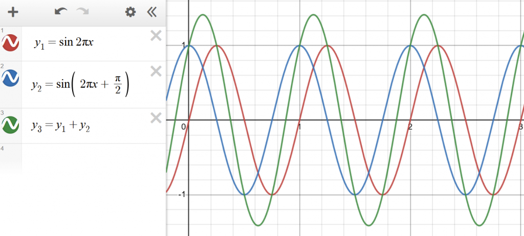
Note that the amplitude of $y_3=y_1+y_2$ is smaller than the sum of amplitude of $y_1$and$y_2$.
Therefore we need to apply the same phase change to the original signal before mixing. The usual practice is to pass through an all-pass filter, i.e. a filter that changes only the phase and not the amplitude. The transfer function of an all-pass filter can be like this:
$H(j\omega) = \frac{ j\omega – \omega_c }{ j\omega + \omega_c }$
And the phase is:
$\theta(\omega)=-2arctan(\frac{\omega}{\omega_{c}})$
With the desired phase shift and frequency domain invariance, we can solve for the all-pass filter corresponding to the given filter.
When the filters are connected in parallel, we often need to unify the phase of the signals first by the corresponding all-pass filters before mixing them.
Note: This iterative filter is an infinite impulse response filter (IIR), where the output at each moment depends on all past moments. The filtering scheme we discarded at the beginning of the section on digital filters, i.e., Fourier transform + frequency domain operation + Fourier inversion, is a finite impulse response filter (FIR). FIR does not produce nonlinear phase shifts, so it is often used in applications with high phase requirements and low performance requirements, such as image processing. For example, image processing.
Distortion
It’s the time for something easier after discussing all those black magic math of frequAfter all this discussion about the black magic of math, it’s time for something easier.
Distortion works in a pretty simple way. As we mentioned in the section on loudness, rock music uses clipping distortion to create special acoustic effects. When the amplitude of a waveform is too large for the system to record, it will cause clipping. Clipping results in changes in the frequency domain, adding a great amount of overtones to the note.
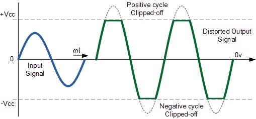
There are two types of clipping. Analog devices are usually using soft cliping. Hard clipping is the easiest one to implement in digital audio.
Compressor
The compressor is similar to an automatic volume controller. When the volume of the input volume is exceeding the threshold, the compressor will compress the audio in a ratio to reduce the volume. When the volume is below the threshold, the compressor will release and does nothing. Compressor reducces the dynamic range of the music. This allows the detailed sound at low volumes to be heard while reducing the peak volume to protect the ear and audio devices.

As you can see in the figure, after a sudden increase in volume, the compressor starts to compress the audio at a predetermined compression ratio; after the audio volume decreases, the compressor stops compressing and releases the volume. The start time and release time are generally called attack and release.
The code implementation is simple. Start the process of attack and turn down the volumn when the volumn exceeds the threshold. Release the compression when the volumn is below the thershold.
Compressors are particularly useful for high dynamic range audio with large changes in loudness.
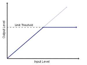
Limiter
Limiter boosts audio volume and avoids distortion caused by clipping. The essence of a limiter is a compressor with a very short start-up time and an infinite compression ratio. Unlike a compressor that always reduces the volume with a fixed ratio, a limiter does not have a fixed compression ratio and will reduce the volume until the volume is less than the system threshold.
In music production, there is a trade-off between volume and dynamic range. If you lose too much dynamic range by maximize loudness, the music will sound very thin.
Delay
The Delay creates a decaying “echo” effect.
The delay interval is generally synchronized with the BPM beat of the song. Let the delay time be T and the intensity ratio between each delay be a, the iterative equation of delay will be:
$Y[t]=X[t]+a*Y[t-T]$
The time complexity of delay effector is $O(n)$.
Since it is using the same iterative structure as the IIR filter, it is possible to perform a filtering process at the same time. In this way, the echoing sound will have a constantly decaying/enhancing frequency band.
Some delay effectors have more complicated functions, such as “ping-pong” delay that bounces between left and right channel.
Reverb
In the real world, audio is constantly reflected as it travels through space. Most of the time the reflected sound reaches the human ears very shortly after the original sound, so the human ear perceives them as a single sound. Reverberation makes the sound thicker, more spatial, and more natural.

The human ear will first receive several early reflections, followed by more reflections and reflections of reflections that travel through space, gradually mix together and decay.
Unlike delays with fixed echo intervals, reverbs are reflections in natural space, which is hard to simultae with simple functions and iterations. Digital reverb effectors usually use convolution of the impulse response function.
Impulse function is also known as Dirac function in physics. The expression of the impulse function is as follows.
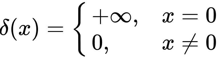
The integral of the impulse function is 1.

In digital signal processing, people usually use the discrete version of Dirac funciton, which is called unit impulse function. It has the following defination:

The impulse function is equivalent to a very short pulse with an intensity of 1. The impulse response function is the response of the system to this impulse. The diagram below is an example of impulse response (small lecture hall reverb):

The response funciton $g(x)$ is the strength of the impluse $t$ seconds after it enters the system.
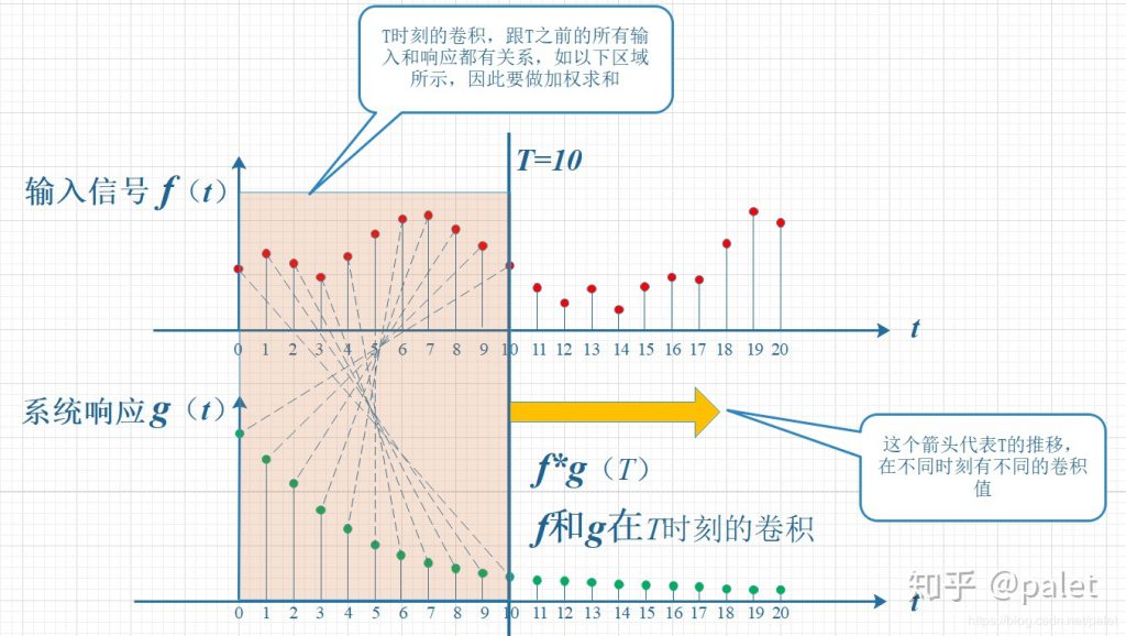
For a discrete signal $f(x)$, the output at moment $t$ is:
$\sum_{n=0}^{\infty} f (t-n) g (n)$
Which means $f (t)*g (0)$ plus $f (t-1)*g (1)$ plus $f (t-2)*g (2)$… etc. Here is a illustratio by Zhihu@palet:
Invert and shift to obtain the convolution expression.
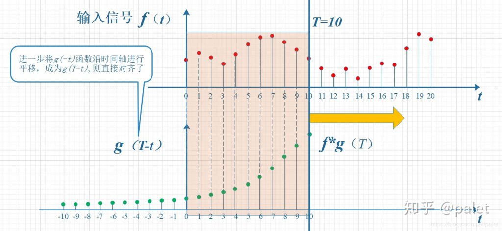
$(f*g)(n)=\sum_{\tau=-\infty }^{\infty}f(\tau)g(n-\tau)$
In practice, the sample length and impulse response function are finite in length. Moreover, the reverberation basically decays to a range that is not audible to the human ear after a period of time appropriately considering the computati. We can reduce the convolution size considering the computational cost.
Reference: